High weak order SDE solvers

This post summarizes our new high weak order methods for the SciML ecosystem, as implemented within the Google Summer of Code 2020 project.

After an introductory part highlighting the differences between the strong and the weak approximation for stochastic differential equations, we look into the convergence and performance properties of a few representative new methods in case of a non-commutative noise process. Based on the stochastic version of the Brusselator equations, we demonstrate how adaptive step-size control for the weak solvers can result in a better approximation of the system dynamics. Finally, we discuss how to run simulations on GPU hardware.

Throughout this post, we shall use the vector notation $X(t)$ to denote the solution of the d-dimensional Ito SDE system

$$ dX(t) = a(t,X(t)) dt + b(t,X(t)) dW $$

with an m-dimensional driving Wiener process W(t) in the time span $\mathbb{I}=[t_0, T]$, where $a: \mathbb{I}\times\mathbb{R}^d \rightarrow \mathbb{R}^d$ and $b: \mathbb{I}\times \mathbb{R}^{d} \rightarrow \mathbb{R}^{d \times m}$ are continuous functions which fulfill a global Lipschitz condition.¹ For simplicity, we write $X(t)$ for both time-discrete approximations and continuous-time random variables in the following.

Strong convergence

Suppose that we encounter the following problem: Given noisy observations $Z(t)$ (e.g., originating from measurement noise), what is the best estimate $\hat{X}(t)$ of a stochastic system $X(t)$ satisfying the form above. Intuitively, we aim at filtering away the noise from the observations in an optimal way. Such tasks are well known as filtering problems.

To solve a filtering problem, we need a solver whose sample paths $Y(t)$ are close to the ones of the stochastic process $X(t)$, i.e., the solver should allow us to reconstruct correctly the numerical solution of each single trajectory of an SDE.

Introducing the absolute error at the final time $T$ as $$ \rm{E}(|X(T) -Y(T)|) \leq \sqrt{\rm{E}(|X(T)-Y(T)|^2)}, $$ we define convergence in the strong sense with order $p$ of a time discrete approximation $Y(T)$ with step size $h$ to the solution $X(T)$ of a SDE at time $T$ if there exists a constant $C$ (independent of $h$) and a constant $\delta > 0$ such that $$ \rm{E}(|X(T) -Y(T)|) \leq C \cdot h^p, $$ for each $h \in [0, \delta]$.

The StochasticDiffEq package contains various state-of-the-art solvers for the strong approximation of SDEs. In most cases, the strong solvers are however restricted to special noise forms. For example, the very powerful stability-optimized, adaptive strong order 3/2 stochastic Runge-Kutta method (SOSRI) can only handle diagonal and scalar noise Ito SDEs, i.e., noise processes where b has only entries on its diagonal or $m=1$. The main difficulty for the construction of strong methods with an order > 1/2 arises from the need of an accurate estimation of multiple stochastic integrals. While the iterated stochastic integrals can be expressed in terms of dW in the case of scalar, diagonal, and commutative noise processes, an approximation based on a Fourier expansion of a Brownian bridge must be employed in the case of non-commutative noise processes.² Currently, we are also implementing those iterated integrals in the StochasticDiffEq library.

Weak convergence

Instead of an accurate pathwise approximation of a stochastic process, we only require an estimation for the expected value of the solution in many situations. In these cases, methods for the weak approximation are sufficient and – due to the less restrictive formulation of the objective – those solvers are computationally cheaper than their strong counterparts. For example, weak solvers are very efficient for simulations in quantum optics, if only mean values of many trajectories are required, e.g., when the expectation values of variables such as position and momentum operators are computed in the phase space framework (Wigner functions, positive P-functions, etc.) of quantum mechanics. Our new contributions are particularly appealing for many-body simulations, which are the computationally most demanding problems in quantum mechanics.

We define convergence in the weak sense with order $p$ of a time-discrete approximation $Y(T)$ with step size $h$ to the solution $X(T)$ of a SDE at time $T$ if there exists a constant $C$ (independent of $h$) and a constant $\delta > 0$ such that $$ |\rm{E}(g(X(T))) -\rm{E}(g(Y(T)))| \leq C \cdot h^p, $$ $~$

for any polynomial $g$ for each $h \in [0, \delta]$.

We demonstrate below that high weak order solvers are specifically appealing, as they allow for using much larger time steps while attaining the same error in the mean, as compared with SDE solvers possessing a smaller weak-order convergence.

New high weak order methods

A list of all new weak solvers is available in the SciML documentation. Note that we also implemented methods designed for the Stratonovich sense. For the subsequent examples regarding Ito SDEs, we use only a subset of the plethora of second-order weak solvers. We employ the DRI1()³, RD1WM()⁴, and RD2WM()⁴ methods due to Debrabant & Rößler and Platen’s PL1WM()¹ method. We compare those methods to the strong Euler-Maruyama EM()¹ and the simplified Euler-Maruyama SimplifiedEM()¹ schemes. The latter is the simplest weak solver, where the Gaussian increments of the strong Euler-Maruyama scheme are replaced by two-point distributed random variables with similar moment properties.

Rößler’s SRK schemes are particularly designed to scale well with the number of Wiener processes m, since only 2m-1 random variables have to be drawn and since the number of function evaluations for the drift and the diffusion terms is independent of m. PL1WM() in contrast needs to simulate m(m+1)/2 random variables but a smaller number of order conditions needs to be fulfilled.

Convergence tests

As in the first blog post, let us consider the multi-dimensional SDE with non-commuting noise³:

$$ \scriptstyle d \begin{pmatrix} X_1 \\ X_2 \end{pmatrix} = \begin{pmatrix} -\frac{273}{512} & \phantom{X_2}0 \\ -\frac{1}{160} \phantom{X_2} & -\frac{785}{512}+\frac{\sqrt{2}}{8} \end{pmatrix} \begin{pmatrix} X_1 \\ X_2 \end{pmatrix} dt + \begin{pmatrix} \frac{1}{4} X_1 & \frac{1}{16} X_1 \\ \frac{1-2\sqrt{2}}{4} X_2 & \frac{1}{10}X_1 +\frac{1}{16} X_2 \end{pmatrix} d \begin{pmatrix} W_1 \\ W_2 \end{pmatrix}
$$

with initial value $$ ~$$

$$ X(t=0)= \begin{pmatrix} 1 \\ 1\end{pmatrix},$$

where the expected value of the solution can be computed analytically

$$ \rm{E}\left[ f(X(t)) \right] = \exp(-t),$$

for the function $f(x)=(x_1)^2$, which we use to test the weak convergence order of the algorithms in the following.

To compute the expected value numerically, we sample an ensemble of numtraj = 1e6 trajectories for different step sizes dt.

using StochasticDiffEq
using Test
using Random
using Plots
using DiffEqDevTools

function prob_func(prob, i, repeat)
    remake(prob,seed=seeds[i])
end

u₀ = [1.0,1.0]
function f1!(du,u,p,t)
  @inbounds begin
    du[1] = -273//512*u[1]
    du[2] = -1//160*u[1]-(-785//512+sqrt(2)/8)*u[2]
  end
  return nothing
end
function g1!(du,u,p,t)
  @inbounds begin
    du[1,1] = 1//4*u[1]
    du[1,2] = 1//16*u[1]
    du[2,1] = (1-2*sqrt(2))/4*u[1]
    du[2,2] = 1//10*u[1]+1//16*u[2]
  end
  return nothing
end
dts = 1 .//2 .^(3: -1:0)
tspan = (0.0,3.0)

h2(z) = z^2 # but apply it only to u[1]

prob = SDEProblem(f1!,g1!,u₀,tspan,noise_rate_prototype=zeros(2,2))

numtraj = Int(1e6)
seed = 100
Random.seed!(seed)
seeds = rand(UInt, numtraj)
ensemble_prob = EnsembleProblem(prob;
        output_func = (sol,i) -> (h2(sol[end][1]),false),
        prob_func = prob_func
        )

sim = test_convergence(dts,ensemble_prob,DRI1(),
  save_everystep=false,trajectories=numtraj,save_start=false,adaptive=false,
  weak_timeseries_errors=false,weak_dense_errors=false,
  expected_value=exp(-3.0)
  )

The object sim defined in the last line contains all relevant quantities to test the weak convergence with respect to the final time point for the DRI1() scheme. Repeating this call to the test_convergence() function for the other aforementioned solvers, we obtain the convergence plot:

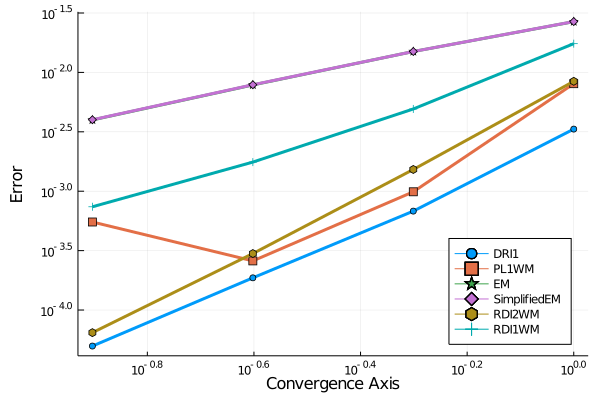
Note that the SimplifiedEM and the EM scheme fall on top of each other. DRI1() achieves the smallest errors for a fixed dt in this study.

Work-Precision Diagrams

Ultimately, we are not only interested in the general convergence slope of an algorithm but also in its speed. We’d like to select the fastest method depending on the permitted tolerance. This is commonly studied using work-precision diagram. Thanks to new routines, a user can generate a work-precision diagram by the following code

reltols = 1.0 ./ 4.0 .^ (1:4)
abstols = reltols#[0.0 for i in eachindex(reltols)]
setups = [
          Dict(:alg=>DRI1(),:dts=>dts,:adaptive=>false),
          Dict(:alg=>PL1WM(),:dts=>dts,:adaptive=>false),
          Dict(:alg=>EM(),:dts=>dts,:adaptive=>false),
          Dict(:alg=>SimplifiedEM(),:dts=>dts,:adaptive=>false),
          Dict(:alg=>RDI2WM(),:dts=>dts,:adaptive=>false),
          Dict(:alg=>RDI1WM(),:dts=>dts,:adaptive=>false)
          ]
test_dt = 1//10000
appxsol_setup = Dict(:alg=>EM(), :dt=>test_dt)
wp = @time WorkPrecisionSet(ensemble_prob,
                            abstols,reltols,setups,test_dt;
                            maxiters = 1e7,verbose=false,
                            save_everystep=false,save_start=false,
                            appxsol_setup = appxsol_setup,
                            expected_value=exp(-3.0),
                            trajectories=numtraj, error_estimate=:weak_final)
plt = plot(wp;legend=:bottomleft)

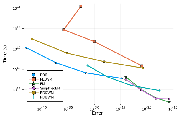
Therefore, DRI1 has the best performance in this non-commutative noise case if the error is supposed to stay below 1e-3. For larger permitted errors, the SimplifiedEM scheme might be a good choice. However, the first order methods are outclassed when high precision is more of a concern. We plan to perform more in-depth benchmarks in the near future what will be reported on the SciML news. Stay tuned!

Adaptive step-size control

Already in 2004, Rößler proposed an adaptive discretization algorithm for the weak approximation of SDEs.⁴ The idea is to employ an embedded SRK scheme: Using the same function evaluations but distinct Butcher tableaus, one constructs two stochastic Runge-Kutta methods with different convergence order, such that the local error can be estimated with only small additional computational overhead. Based on the error estimate, new step sizes are proposed.

To use adaptive step-size control, it is sufficient to set adaptive=true (default setting). Optionally, one may also pass absolute and relative tolerances.

The following julia code simulates the stochastic version of the Brusselator equations with intitial condition

$$ X(t=0)= \begin{pmatrix} 0.1 \\ 0\end{pmatrix},$$

on a time span $\mathbb{I}=[0, 100]$ for adaptive (sol) and fixed step sizes (sol_na):

using StochasticDiffEq, DiffEqNoiseProcess, Random
using Plots
using DiffEqGPU

function prob_func(prob, i, repeat)
  Random.seed!(seeds[i])
  W = WienerProcess(0.0,0.0,0.0)
  remake(prob,noise=W)
end

function brusselator_f!(du,u,p,t)
  @inbounds begin
    du[1] = (p[1]-1)*u[1]+p[1]*u[1]^2+(u[1]+1)^2*u[2]
    du[2] = -p[1]*u[1]-p[1]*u[1]^2-(u[1]+1)^2*u[2]
  end
  nothing
end

function scalar_noise!(du,u,p,t)
  @inbounds begin
    du[1] = p[2]*u[1]*(1+u[1])
    du[2] = -p[2]*u[1]*(1+u[1])
   end
   nothing
end


# fix seeds
seed = 100
Random.seed!(seed)
numtraj= 100
seeds = rand(UInt, numtraj)
W = WienerProcess(0.0,0.0,0.0)


u0 = [-0.1f0,0.0f0]
tspan = (0.0f0,100.0f0)
p = [1.9f0,0.1f0]

prob = SDEProblem(brusselator_f!,scalar_noise!,u0,tspan,p,noise=W)

ensembleprob = EnsembleProblem(prob, prob_func = prob_func)

sol = @time solve(ensembleprob,DRI1(),dt=0.1,EnsembleCPUArray(),trajectories=numtraj)
sol_na = @time solve(ensembleprob,DRI1(),dt=0.8,adaptive=false,EnsembleCPUArray(),trajectories=numtraj)


summ = EnsembleSummary(sol,0.0f0:0.5f0:100f0)
pl = plot(summ,fillalpha=0.5,xlabel = "time t", yaxis="X(t)", label= ["x₁(t)" "x₂(t)"], legend=true)

The time evolution of both dependent variables ($x_1(t)$ and $x_2(t)$) displays damped oscillations.

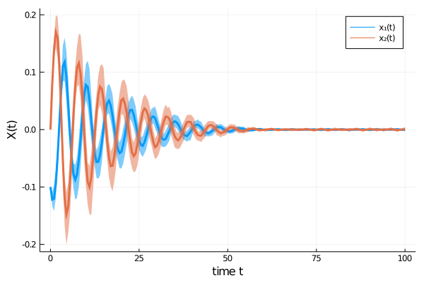
We can confirm Rößler’s observation⁴ that the adaptive scheme describes the time evolution of the SDE more accurately, as oscillations are damped out stronger for the fixed step size method, thus approaching the origin too rapidly.

using DifferentialEquations.EnsembleAnalysis
meansol = timeseries_steps_mean(sol)
meansol_na = timeseries_point_mean(sol_na,meansol.t)
dts = []
tmp1 = tspan[1]
for tmp2 in meansol.t
  global tmp1
  push!(dts,tmp2-tmp1)
  tmp1 = tmp2
end
#

list_plots = []
for i in 1:length(meansol.u)
  l = @layout [a  b]
  plt1 = plot(meansol[1, 1:i],meansol[2, 1:i],
         ylim = (-0.18, 0.18),
         xlim = (-0.13, 0.13),
         xlabel = "x₁(t)",
         yaxis= "x₂(t)",
         label="adaptive",
         lw=2,
         linecolor=1
         )
  plot!(meansol_na[1, 1:i],meansol_na[2, 1:i],
         ylim = (-0.18, 0.18),
         xlim = (-0.13, 0.13),
         xlabel = "x₁(t)",
         yaxis= "x₂(t)",
         label="fixed step size",
         lw=2,
         linecolor=2
         )
  pl2 = scatter(dts[1:i], xlabel = "step", yaxis= "dtᵢ", xlim = (0, length(meansol.u)),  ylim = (0.0, 2.3), legend=false)
  plt = plot(plt1, pl2, layout = l)
  push!(list_plots, plt)
end

anim = animate(list_plots,lw=2,every=1)

GPU usage

All necessary tools to accelerate the simulation of (stochastic) differential equations on GPUs within the SciML ecosystem are collected in the DiffEqGPU package.

Currently, bounds checking and return values are not allowed, i.e., functions must be written in the form:

function f!(du,u,p,t)
  @inbounds begin
    du[1] = ..
  end
  nothing
end

Except from those limitations, a user can specifiy ensemblealg=EnsembleGPUArray() to parallelize SDE solves across the GPU, see, e.g., the GPU tests for StochasticDiffEq for some examples. Note that for some high weak order solvers GPU usage is not recommended as scalar indexing is used.

If you have any questions or comments, please don’t hesitate to contact me!