Neural Hybrid Differential Equations

I am delighted that I have been awarded my second GSoC stipend this year. I look forward to carrying out the ambitious project scope with my mentors Chris Rackauckas, Moritz Schauer, Yingbo Ma, and Mohamed Tarek. This year’s project is embedded within the NumFocus/SciML organization and comprises adjoint sensitivity methods for discontinuities, shadowing methods for chaotic dynamics, symbolically generated adjoint methods, and further AD tooling within the Julia Language.

This first post aims to illustrate our new (adjoint) sensitivity analysis tools with respect to event handling in (ordinary) differential equations (DEs).

Note: Please check the SciMLSensitivity.jl docs for a maintained neural hybrid DE tutorial!

Hybrid Differential Equations

DEs with additional explicit or implicit discontinuities are called hybrid DEs. Within the SciML software suite, such discontinuities may be incorporated into DE models by callbacks. Evidently, the incorporation of discontinuities allows a user to specify changes (events) in the system, i.e., changes of the state or the parameters of the DE, which cannot be modeled by a plain ordinary DE. While explicit events can be described by DiscreteCallbacks, implicit events have to be specified by ContinuousCallbacks. That is, explicit events possess explicit event times, while implicit events are triggered when a continuous function evaluates to 0. Thus, implicit events require some sort of rootfinding procedure.

Some relevant examples for hybrid DEs with discrete or continuous callbacks are:

• quantum optics experiments, where photon-counting measurements lead to jumps in the quantum state that occur with a variable rate, see for instance Appendix A in Ref.¹ (ContinuousCallback).
• a bouncing ball² (ContinuousCallback).
• classical point process models, such as a Poisson process³.
• digital controllers⁴, where a continuous system dynamics is controlled by a discrete-time controller (DiscreteCallback).
• pharmacokinetic models⁵, where explicit dosing times change the drug concentration in the blood (DiscreteCallback). The simplest possible example being the one-compartment model.
• kicked oscillator dynamics, e.g., a harmonic oscillator that gets a kick at some time points (DiscreteCallback).

The associated sensitivity methods that allow us to differentiate through the respective hybrid DE systems have been recently introduced in Refs. ² and ³.

Kicked harmonic oscillator

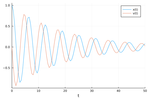
Let us consider the simple physical model of a damped harmonic oscillator, described by an ODE of the form

$$ \ddot{x}(t) + a\cdot\dot{x}(t) + b \cdot x(t) = 0 , $$

where $a=0.1$ and $b=1$ with initial conditions

$$ \begin{aligned} x(t=0) &= 1 \\ v(t=0) &= \dot{x}(t=0) = 0. \end{aligned}
$$

This second-order ODE can be reduced to two first-order ODEs, such that we can straightforwardly simulate the resulting ODE with the DifferentialEquations.jl package. (Instead of doing this reduction manually, we could also use ModelingToolkit.jl to transform the ODE in an automatic manner. Alternatively, for second-order ODEs, there is also a SecondOrderODEProblem implemented.) The Julia code reads:

using DiffEqFlux, DifferentialEquations, Flux, Optim, Plots, DiffEqSensitivity
using Zygote
using Random
u0 = Float32[1.; 0.]

tspan = (0.0f0,50.0f0)

dtsave = 0.5f0
t = tspan[1]:dtsave:tspan[2]

function oscillator!(du,u,p,t)
  du[1] = u[2]
  du[2] = - u[1] - 1//10*u[2]
  return nothing
end

prob_data = ODEProblem(oscillator!,u0,tspan)

# ODE without kicks
pl = plot(solve(prob_data,Tsit5(),saveat=t), label=["x(t)" "v(t)"])

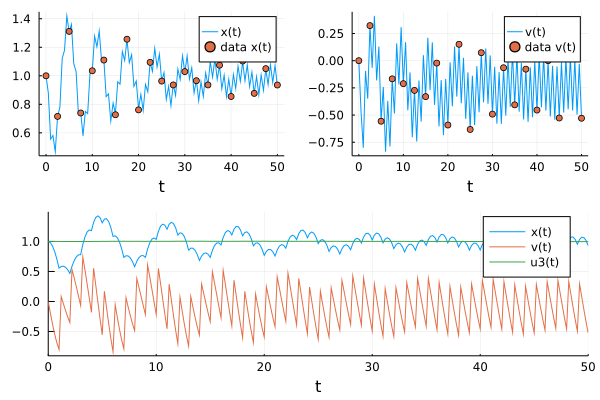
We now include a kick to the velocity of the oscillator at regular time steps. Here, we choose both the time difference between the kicks and the increase in velocity as 1.

kicktimes = tspan[1]:1:tspan[2]
function kick!(integrator)
  integrator.u[end] += one(eltype(integrator.u))
end
cb_ = PresetTimeCallback(kicktimes,kick!,save_positions=(false,false))

sol_data = solve(prob_data,Tsit5(),callback=cb_,saveat=t)
t_data = sol_data.t
ode_data = Array(sol_data)

# visualize data
pl1 = plot(t_data,ode_data[1,:],label="data x(t)")
plot!(pl1,t_data,ode_data[2,:],label="data v(t)")

pl2 = plot(t_data[1:20],ode_data[1,1:20],label="data x(t)")
plot!(pl2,t_data[1:20],ode_data[2,1:20],label="data v(t)")
pl = plot(pl2, pl1, layout=(1,2), xlabel="t")

High domain knowledge

For simplicity, we assume that we have almost perfect knowledge about our system. That is, we assume to know the basic structure of the ODE, including its parameters $a$ and $b$, and that the affect! function of the event only acts on the velocity. We then encode the affect as an additional component to the ODE. The task is thus to learn the dynamics of the third component of integrator.u. If we further set the initial value of that component to 1, then the neural network only has to learn that du[3] is 0. In other words, the output of the neural network must be 0 for all states u.

Random.seed!(123)
nn1 = FastChain(FastDense(2, 64, tanh),FastDense(64, 1))
p_nn1 = initial_params(nn1)

function f1!(du,u,p,t)
  du[1] = u[2]
  du[2] = - u[1] - 1//10*u[2]
  du[3] = nn1(u[1:2], p)[1]
  return nothing
end

affect!(integrator) = integrator.u[2] += integrator.u[3]
cb = PresetTimeCallback(kicktimes,affect!,save_positions=(false,false))
z0 = Float32[u0;one(u0[1])]
prob1 = ODEProblem(f1!,z0,tspan,p_nn1)

We can easily compare the time evolution of the neural hybrid DE with respect to the data:

# to visualize the predictions of the trained neural network below
function visualize(prob,p)
  _prob = remake(prob,p=p)
  ode_pred = Array(solve(_prob,Tsit5(),callback=cb,
                 saveat=dtsave))[1:2,:]
  pl1 = plot(t_data,ode_pred[1,:],label="x(t)")
  scatter!(pl1,t_data[1:5:end],ode_data[1,1:5:end],label="data x(t)")
  pl2 = plot(t_data,ode_pred[2,:],label="v(t)")
  scatter!(pl2,t_data[1:5:end],ode_data[2,1:5:end],label="data v(t)")

  pl = plot(pl1, pl2, layout=(1,2), xlabel="t")
  return pl, sum(abs2,ode_data .- ode_pred)
end

pl = plot(solve(prob1,Tsit5(),saveat=t,
  callback=cb
  ),label=["x(t)" "v(t)" "u3(t)"])

which (of course) doesn’t match the data due to the random initialization of the neural network parameters before training. The neural network can be trained, i.e., its parameters can be optimized, by minimizing a mean-squared error loss function:

### loss function
function loss(p; prob=prob1, sensealg = ReverseDiffAdjoint())
  _prob = remake(prob,p=p)
  pred = Array(solve(_prob,Tsit5(),callback=cb,
               saveat=dtsave,sensealg=sensealg))[1:2,:]
  sum(abs2,ode_data .- pred)
end

loss(p_nn1)

The recently implemented tools are deeply hidden within the DiffEqSensitivity.jl package. However, while the user could previously only choose discrete sensitivities such as ReverseDiffAdjoint() or ForwardDiffAdjoint() that rely on direct differentiation through the solver operations to get accurate gradients, one can now also select continuous adjoint sensitivity methods such as BacksolveAdjoint(), InterpolatingAdjoint(), and QuadratureAdjoint() as the sensealg for hybrid DEs. Each choice has its own characteristics in terms of stability, scaling with parameters, and memory consumption, see, e.g., Chris’ talk at the SciML symposium at SIAM CSE.

###################################
# training loop
# optimize the parameters for a few epochs with ADAM
function train(prob, p_nn; sensealg=BacksolveAdjoint())
  opt = ADAM(0.0003f0)
  list_plots = []
  losses = []
  for epoch in 1:200
    println("epoch: $epoch / 200")
    _dy, back = Zygote.pullback(p -> loss(p,
      prob=prob,
      sensealg=sensealg), p_nn)
    gs = @time back(one(_dy))[1]
    push!(losses, _dy)
    if epoch % 10 == 0
      # plot every xth epoch
      pl, test_loss = visualize(prob, p_nn)
      println("Loss (epoch: $epoch): $test_loss")
      display(pl)
      push!(list_plots, pl)
    end
    Flux.Optimise.update!(opt, p_nn, gs)
    println("")
  end
  return losses, list_plots
end

# plot training loss
losses, list_plots = train(prob1, p_nn1)
pl1 = plot(losses, lw = 1.5, xlabel = "epoch", ylabel="loss", legend=false)
pl2 = list_plots[end]
pl3 = plot(solve(prob1,p=p_nn1,Tsit5(),saveat=t,
   callback=cb
  ), label=["x(t)" "v(t)" "u3(t)"])

pl = plot(pl2,pl3)

We see the expected constant value of u[3], indicating a kick to the velocity of +=1, at the kicking times over the full time interval.

Reducing the domain knowledge

If less physical information is included in the model design, the training becomes more difficult, e.g., due to local minima. Possible modification for the kicked oscillator could be

• changing the initial condition of the third component of u,
• using another affect function affect!(integrator) = integrator.u[2] = integrator.u[3],
• dropping the knowledge that only u[2] gets a kick by using a neural network with 2 outputs (+ a fourth component in the ODE):

affect2!(integrator) = integrator.u[1:2] = integrator.u[3:4]
function f2!(du,u,p,t)
  du[1] = u[2]
  du[2] = - u[1] - 1//10*u[2]
  du[3:4] .= nn2(u[1:2], nn_weights)
  return nothing
end

• fitting the parameters $a$ and $b$ simultaneously:

function f3!(du,u,p,t)
  a = p[end-1]
  b = p[end]
  nn_weights = p[1:end-2]

  du[1] = u[2]
  du[2] = -b*u[1] - a*u[2]
  du[3:4] .= nn2(u[1:2], nn_weights)
  return nothing
end

• inferring the entire underlying dynamics using a neural network with 4 outputs:

function f4!(du,u,p,t)
  Ω = nn3(u[1:2], p)

  du[1] = Ω[1]
  du[2] = Ω[2]
  du[3:4] .= Ω[3:4]
  return nothing
end

• etc.

Outlook

With respect to the adjoint sensitivity methods for hybrid DEs, we are planning to

• refine the adjoints in case of implicit discontinuities (ContinuousCallbacks) and
• support direct usage through the jump problem interface

in the upcoming weeks. For further information, the interested reader is encouraged to look at the open issues in the DiffEqSensitivity.jl package.

If you have any questions or comments, please don’t hesitate to contact me!