Sensitivity Analysis of Hybrid Differential Equations

In this post, we discuss sensitivity analysis of differential equations with state changes caused by events triggered at defined moments, for example reflections, bounces off a wall or other sudden forces. These are described by hybrid differential equations¹. We highlight differences between explicit² and implicit events^{3 4}. As a paradigmatic example, we consider a bouncing ball described by the ODE

$$ \begin{aligned} \text{d}z(t) &= v(t) \text{d}t, \\ \text{d}v(t) &= -\mathrm g\thinspace \text{d}t \end{aligned}
$$

with initial condition

$$ \begin{aligned} z(t=0) &= z_0 = 5, \\ v(t=0) &= v_0 = -0.1. \end{aligned}
$$

The initial condition contains the initial height $z_0$ and initial velocity $v_0$ of the ball. We have two important parameters in this system. First, there is the gravitational constant $\mathrm g=10$ modeling the acceleration of the ball due to an approximately constant gravitational field.

Second, we model the ground as barrier at $z = 0$ where the ball bounces off in opposite direction. We include a dissipation factor $\gamma=0.8$ (coefficient of restitution) that accounts for a imperfect elastic bounce on the ground.

When ignoring the bounces, we can straightforwardly integrate the ODE analytically

$$ \begin{aligned} z(t) &= z_0 + v_0 t - \frac{\mathrm g}{2} t^2, \\ v(t) &= v_0 - \mathrm g\thinspace t \end{aligned}
$$

or numerically using the OrdinaryDiffEq package from the SciML ecosystem.

### simulate forward

using ForwardDiff, Zygote, OrdinaryDiffEq, DiffEqSensitivity
using Plots, LaTeXStrings

# dynamics
function f(du,u,p,t)
  du[1] = u[2]
  du[2] = -p[1]
end

# parameters and solve
z0 = 5.0
v0 = -0.1
t0 = 0.0
tend = 1.9
g = 10
γ = 0.8

u0 = [z0,v0]
tspan = (t0,tend)
p = [g, γ]
prob = ODEProblem(f,u0,tspan,p)

# plot forward trajectory
sol = solve(prob,Tsit5(),saveat=0.1)
pl = plot(sol, label = ["z(t)" "v(t)"], labelfontsize=20, legendfontsize=20, lw = 2, xlabel = "t", legend=:bottomleft)
hline!(pl, [0.0], label=false, color="black")
savefig(pl,"BB_forward_no_bounce.png")

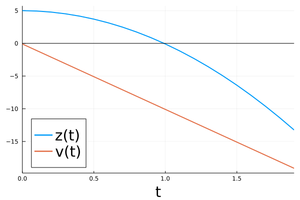
Of course, this way the ball continues to fall through the barrier at $z=0$.

Forward simulation with events

At time $\tau$ around $\tau \approx 1$, the ball hits the ground $z(\tau) = 0$, and is inelastically reflected while dissipating a fraction of its energy. This can be modeled by re-initializing the ODE at time $\tau$ with new initial conditions

$$ \begin{aligned}
z({\tau}) &= z(\tau-) ,\\ v({\tau})&= -\gamma v(\tau-) , \end{aligned}
$$

so that there is a jump in the velocity at the event time: the velocity right before the bounce, the left limit $v(\tau-)$, and the velocity with which the ball continues its movement after the bounce $v(\tau)$, are different.

Given our analytical solution for the state as a function of time, we can easily compute the event time $\tau$ in terms of the initial condition and parameters as

$$ \tau = \frac{v_0 + \sqrt{v_0^2 + 2 \mathrm g z_0}}{\mathrm g}. $$

Explicit events

We can define the bounce of the ball as an explicit event by inserting the values of the initial condition and the parameters into the formula for $\tau$. We obtain

$$ \tau = 0.99005. $$

The full explicit trajectory $z_{\rm exp}(t) = z(t)$ is determined by

$$ z(t) = \begin{cases} z_0 + v_0 t - \dfrac{\mathrm g}{2} t^2 ,& \forall t < \tau, \\ -0.4901 \mathrm g - 0.5 \mathrm g (-0.99005 + t)^2 + 0.99005 v_0 + z_0\\ \quad - (-0.99005 + t) (-0.99005 \mathrm g + v_0)\gamma ,& \forall t \ge \tau, \end{cases} $$

where we used

$$ \begin{aligned}
z({\tau})&= z_0 + 0.99005 v_0 -0.4901 \mathrm g, \\ v({\tau})&= -\gamma v({\tau-}) = -\gamma(v_0 - 0.99005 \mathrm g) . \end{aligned}
$$

Here the change in state $(z,v)$ at the event time is defined with the help of an affect function

$$ a(z,v) = (z, -\gamma v). $$

Numerically, we use a DiscreteCallback in this case to simulate the system.

# solve with DiscreteCallback (explicit event)
tstar = (v0 + sqrt(v0^2+2*z0*g))/g
condition1(u,t,integrator) = (t == tstar)
affect!(integrator) = integrator.u[2] = -integrator.p[2]*integrator.u[2]
cb1 = DiscreteCallback(condition1,affect!,save_positions=(true,true))

sol1 = solve(prob,Tsit5(),callback=cb1, saveat=0.1, tstops=[tstar])

Evidently, by choosing an explicit definition of the event, the impact time is fixed. The reflection event is triggered at $\tau = 0.99005$, a time where under different initial configurations the ball perhaps hasn’t reached the ground.

Implicit events

The physically more meaningful description of a bouncing ball is therefore given by an implicit description of the event in form of a condition (event function)

$$ g(z,v,p,t), $$

where an event occurs at time $\tau$ if $g(z(\tau),v(\tau),p,\tau) = 0$. We have already used this condition to define our impact time $\tau$ when modeling the bounce explicitly. The implicit formulation also lends itself to take multiple bounces into account by triggering the event every time $g(z,v,p,t) = 0$.

As in the previous case, we can analytically compute the full trajectory of the ball. By substituting the formula for $\tau$ we have at the event time

\begin{aligned} z({\tau})&= 0, \\ v({\tau}-)&= - \sqrt{v_0^2 + 2 \mathrm g z_0} \end{aligned}

for the left limit and

\begin{aligned} v({\tau})&= \gamma \sqrt{v_0^2 + 2 \mathrm g z_0} \end{aligned}

right after the bounce. Thus, the full trajectory $z_{\rm imp}(t) = z(t)$ is given by

$$ (\star) \quad z(t) = \begin{cases} z_0 + v_0 t - \dfrac{\mathrm g}{2} t^2 ,& \forall t < \tau ,\\ -\dfrac{-\mathrm g t + v_0 + \sqrt{v_0^2 + 2 \mathrm g z_0}}{2 \mathrm g} \\ \quad\cdot \space (-\mathrm g t + v_0 + \sqrt{v_0^2 + 2 \mathrm g z_0} (1 + 2 \gamma)), & \forall t \ge \tau. \end{cases} $$

This is correct even if one substitutes, e.g., a value with higher precision $\mathrm g = 9.81$ for the gravitation constant.

Numerically, we use a ContinuousCallback in this case.

# solve with ContinuousCallback (implicit event)
condition2(u,t,integrator) = u[1] # Event happens when condition2(u,t,integrator) == 0
cb2 = ContinuousCallback(condition2,affect!,save_positions=(true,true))
sol2 = solve(prob,Tsit5(),callback=cb2,saveat=0.1)

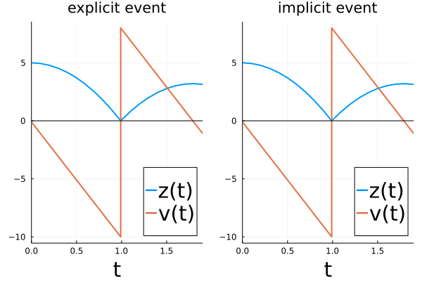
We can verify that both callbacks lead to the same forward time evolution (for fixed initial conditions and parameters).

# plot forward trajectory
pl1 = plot(sol1, label = ["z(t)" "v(t)"], title="explicit event", labelfontsize=20, legendfontsize=20, lw = 2, xlabel = "t", legend=:bottomright)
pl2 = plot(sol2, label = ["z(t)" "v(t)"], title="implicit event", labelfontsize=20, legendfontsize=20, lw = 2, xlabel = "t", legend=:bottomright)
hline!(pl1, [0.0], label=false, color="black")
hline!(pl2, [0.0], label=false, color="black")
pl = plot(pl1,pl2)
savefig(pl,"BB_forward.png")

In addition, the implicitly defined impact time via the ContinuousCallback also changes appropriately when changing the initial conditions or the parameters, for example when using $\mathrm g = 9.81$ for the gravitation constant. In other words, the event time $\tau=\tau(p,z_0,v_0,t_0)$ is a function of the parameters and initial conditions, and is implicitly defined by the event condition.

Suppose we let the ball drop from a somewhat higher position now. Does an increase in height $z$ at $t=0$ give an increase or decrease in height at the end time $t_\text{end}=1.9$? This is something we can answer with sensitivity analysis. For example if we increase the height by (a fraction of) one unit then using $(\star)$

$$ \frac{\text{d} z(t_\text{end})}{\text{d} z_0} = 0.84, $$

meaning the height at $t_\text{end}$ is also by a corresponding fraction of 0.84 units higher.

We can verify this visually:

# animate forward trajectory
sol3 = solve(remake(prob,u0=[u0[1]+0.5,u0[2]]),Tsit5(),callback=cb2,saveat=0.01)

plt2 = plot(sol2, label = false, labelfontsize=20, legendfontsize=20, lw = 1, xlabel = "t", legend=:bottomright, color="black", xlims=(t0,tend))
hline!(plt2, [0.0], label=false, color="black")
plot!(plt2, sol3, tspan=(t0,tend), color=[1 2], label = ["z(t)" "v(t)"], labelfontsize=20, legendfontsize=20, lw = 2, xlabel = "t", legend=:bottomright, denseplot=true, xlims=(t0,tend), ylims=(-11,9))
# scatter!(plt2, [t2,t2], sol3(t2), color=[1, 2], label=false)

list_plots = []
for t in sol3.t
  tstart = 0.0

  plt1 = plot(sol2, label = false, labelfontsize=20, legendfontsize=20, lw = 1, xlabel = "t", legend=:bottomright, color="black")
  hline!(plt1, [0.0], label=false, color="black")
  plot!(plt1, sol3, tspan=(t0,t), color=[1 2], label = ["z(t)" "v(t)"], labelfontsize=20, legendfontsize=20, lw = 2, xlabel = "t", legend=:bottomright, denseplot=true, xlims=(t0,tend), ylims=(-11,9))
  scatter!(plt1,[t,t], sol3(t), color=[1, 2], label=false)
  plt = plot(plt1,plt2)
  push!(list_plots, plt)
end

plot(list_plots[100])

anim = animate(list_plots,every=1)

The original curve is shown in black in the figure above.

Sensitivity analysis with events

In more general terms, the last example can be seen as a loss function acting on $z$ at the end time

$$ L^{\text{exp}} = z(t_{\text{end}}), $$

where the superscript “exp” refers to an explicit definition of the time ($t_{\text{end}}$) at which we evaluate the loss function. Let $\alpha$ denote any of the inputs $(z_0,v_0,g,\gamma)$. The sensitivity with respect to $\alpha$ is then given by the chain rule

$$ \frac{\text{d}L^{\text{exp}}}{\text{d} \alpha} = \frac{\text{d}L^{\text{exp}}}{\text{d} z} \frac{\text{d}z(t_{\text{end}})}{\text{d} \alpha} = \frac{\text{d}z(t_{\text{end}})}{\text{d} \alpha}. $$

Inserting our results for $z(t) = z_{\rm exp}(t)$ instead of $z(t) = z_{\rm imp}(t)$ at $t_{\text{end}}$, a different value for the sensitivity is obtained (a value ignoring the changes in $z$ due to changes in the bouncing time $\tau$), e.g.,

$$ \quad \frac{\text{d}L^{\text{exp}}}{\text{d} z_0} = \begin{cases} 1 & \text{with } z(t) = z_{\rm exp}(t) ,\\ 0.84 & \text{with } z(t) = z_{\rm imp}(t) . \end{cases} $$

Besides an explicit description of time points, we may also encounter implicitly defined time points. For example, for the bouncing ball with velocity at the impact time $\tau-$ (i.e., at the left limit) as the quantity of interest,

$$ L = v(\tau-), $$

we could be interested in the sensitivity of $L$ with respect $g$. Using the velocity $v(t)$ at the explicit time $t = 0.9905$ instead of the implicit $v(\tau-)$, again a different value for the sensitivity is obtained (a value again ignoring the changes in $\tau$ and not the one we are looking for), even though $\tau = 0.9905$ in both cases:

$$ \quad \frac{\text{d}L}{\text{d} g} = \begin{cases} -0.99005 & \text{with } v(t) = v_{\rm exp}(t) ,\\ -\frac{g}{\sqrt{v_0^2 + 2 g z_0}} = -0.99995 & \text{ with } v(t) = v_{\rm imp}(t) . \end{cases} $$

Thanks to our analytical results for the bouncing ball, the sensitivity computation has been straightforward up to now. However, in most systems, we won’t be able to solve analytically a differential equation

$$ \text{d}x(t) = f(x,p,t) \text{d}t $$

with initial condition $x_0=x(t_0)$. Instead, we have to numerically solve for the trajectory $x(t)$.

More completely, we will in the following derive an adjoint sensitivity method for a loss function

$$L = \sum_j L_j(\tau_j,x(\tau_j),p) + \sum_i L^{\text{exp}}_i(s_j,x(s_i),p) ,$$

with $L_i^{\text{exp}}$ at explicit time points $s_i$, such as $t_{\text{end}}$, and $L_j(\tau_j,x(\tau_j),p)$ at implicit time points, such as $\tau$, which allows us to compute the sensitivity of $L$ with respect to changes of the parameters or initial condition without the requirement of an analytical solution for $x(t)$.

Backsolve-Adjoint algorithm for ordinary differential equations

Taking derivatives (or finding sensitivities) works in a beautiful mechanical way. We or a computer can find the derivatives of complex expressions by just repeatedly applying the chain rule.

We write

$$\text{solve}(t_0, x_0, t, p)$$

$(= x(t))$ for the functional solution of the ODE at time $t$.

Regarding the computation of the sensitivities (the derivatives of the function solve), we may then choose one of the available algorithms for the given differential equation. Currently, BacksolveAdjoint(), InterpolatingAdjoint(), QuadratureAdjoint(), ReverseDiffAdjoint(), TrackerAdjoint(), and ForwardDiffAdjoint() are compatible with events in ordinary differential equations.

Let us focus on the BacksolveAdjoint() algorithm which computes the sensitivities

$$ \begin{aligned} \frac{\text{d}\thinspace L(\text{solve}(t_0, x_0, t, p))}{\text{d}x_{0}} &= \lambda(t_{0}),\\ \frac{\text{d}\thinspace L(\text{solve}(t_0, x_0, t, p))}{\text{d}p} &= \lambda_{p}(t_{0}), \end{aligned} $$

of a loss function $L$ acting on the final state with respect to the initial state and the parameters. It does so by solving an ODE for $\lambda(s)$ in reverse time from $t$ to $t_0$

$$ \begin{aligned} \frac{\text{d}\lambda(s)}{\text{d}s} &= -\lambda(s)^\dagger \frac{\text{d} f(\rightarrow x(s), p, t)}{\text{d} x(s)} \\ \frac{\text{d}\lambda_{p}(s)}{\text{d}s} &= -\lambda(s)^\dagger \frac{\text{d} f(x(s), \rightarrow p, s)}{\text{d} p}, \end{aligned} $$

with initial conditions:

$$ \begin{aligned} \lambda(t)&= \frac{\text{d}\thinspace L(\text{solve}(t_0, x_0, t, p))}{\text{d}x_{T}}, \\ \lambda_{p}(t) &= 0. \end{aligned} $$

The arrows ($\rightarrow$) indicate the variable with respect to which we differentiate, which will become important later when the same variable shows up in multiple function arguments.

Note that computing the vector-Jacobian products (vjp) in the adjoint ODE requires the value of $x(s)$ along its trajectory. In BacksolveAdjoint(), we recompute $x(s)$ – together with the adjoint variables – backwards in time starting with its final value $x(t)$. A derivation of the ODE adjoint is given in Chris’ MIT 18.337 lecture notes.

BacksolveAdjoint(), essentially the custom primitive differentiation rule of solve, is the elementary building block needed to derive sensitivities also in more complicated examples:

Consider a loss depending on the state $x(s_i)$ at fix time points $s_i$ through loss functions $L_i^{\text{exp}}$,

$$ L^{\text{exp}} = \sum_i L_i^{\text{exp}}(s_i, x(s_i), p). $$

Without contortions we can obtain the sensitivity of $L^{\text{exp}}$ in $p$ (or in $x_0$) using the tool we have. For those a bit familiar with automatic differentiation, this is perhaps easiest to see if we write $L^{\text{exp}}$ as pseudo code

function loss(t0, x0, p)
    x1 = solve(t0, x0, s1, p)
    L = L1(s1, x1, p)
    x2 = solve(s1, x1, s2, p)
    L += L2(s2, x2, p)
    ...
    return L
end

and consider the problem of automatically differentiating it. You’ll just need the primitives of solve, L1 and L2! The sensitivities can be computed by repeated calls to BacksolveAdjoint() on the intervals (s_i, s_{i+1}) backward in time, taking in the sensitivities $\sum_i L^{\text{exp}}(s_i, x(s_i), p)$ at times $s_i$, or according to the common notation² as single call BacksolveAdjoint() with discrete callbacks:

$$ \begin{aligned} \frac{\text{d}\lambda(t)}{\text{d}t} &= -\lambda(t)^\dagger \frac{\text{d} f(\rightarrow x(t), p, t)}{\text{d} x(t)} - \frac{\text{d} L_i^{\text{exp}}(\rightarrow x(t), p)}{\text{d} x(t)}^\dagger \delta(t-s_i), \\ \frac{\text{d}\lambda_{p}(t)}{\text{d}t} &= -\lambda(t)^\dagger \frac{\text{d} f(x(t), \rightarrow p, t)}{\text{d} p} - \frac{\text{d} L_i^{\text{exp}}( x(t),\rightarrow p)}{\text{d} p}^\dagger \delta(t-s_i). \end{aligned} $$

The sensitivities of the ordinary solve with respect to the other arguments are also needed and given by

$$ \frac{\text{d}(\text{solve}(s, x, \rightarrow t, p))}{\text{d}t} = f(\text{solve}(s, x, t, p), p, t) $$

and

$$ \frac{\text{d}(\text{solve}(\rightarrow s, x, t, p))}{\text{d}s} = -f(x, p, s). $$

Now we can even properly define the rrule of solve in the sense of DiffRules.jl.

Explicit events

To make BacksolveAdjoint() compatible with explicit events²,

function loss(t0, x0, p)
    x1- = solve(t0, x0, s1, p)
    L = L1-(s1, x1-, p) # saved before affect
    x1 = a(x1-, p, s1) # affect
    L += L1(s1, x1, p) # saved after affect
    x2- = solve(s1, x1, s2, p)
    L += L2-(s2, x2-, p)
    x2 = a(x2-, p, s2) # affect
    L += L2(s2, x2, p)
    ...
    return L
end

we have to store the event times $s_j$ as well as the state $x(s_j-)$ at the left limit of $s_i$.⁵ We then solve the adjoint ODE backwards in time between the events. As soon as we reach an event time $s_j$ from the right, we update the augmented state according to

$$ \begin{aligned} \lambda({s_j}-) &= \lambda({s_j})^\dagger \frac{\text{d} a(\rightarrow x({s_j}-), p, {s_j}-)}{\text{d} x(s_j-)} \\ \lambda_p({s_j}-) &= \lambda_p({s_j}) - \lambda({s_j})^\dagger \frac{\text{d} a(x({s_j}-), \rightarrow p, {s_j}-)}{\text{d} p} \end{aligned} $$

where $a$ is the affect function applied at the discontinuity. That is, to lift the adjoint from the right to the left limit, we compute a vjp with the adjoint $\lambda({s_j})$ from the right and the Jacobian of the affect function evaluated immediately before the event time at $s_j-$ .

In particular, we apply a loss function callback before and after this update if the state was saved in the forward evolution and entered directly into the loss function.

Implicit events

With implicit events it is similar: Being able to differentiate the ODE when an implicit event terminates the ODE gives us the custom primitive differentiation rule of a solve with implicit callback.

We have to account for an important change: besides the value $\xi = x(\tau)$ at time of the implicit event, the solver returns the variable event time $\tau$ itself.

We could write for an event condition function $g$

$$(\tau_1, \xi_1) = \text{solve2}(t_0, x_0, g, p)$$

to put emphasis on this, or equivalently, compute for a unspecified function $L(t, x, p)$ the result of $\frac{\text{d}L}{\text{d}p}$ with

$$ \begin{aligned} \frac{\text{d}L}{\text{d}p} &= \frac{\text{d}L( \text{solve2}(t_0, x_0, g, \rightarrow p),\rightarrow p)}{\text{d}p}\\ &= \frac{\text{d}L(\tau_1({\color{black}\rightarrow} p), \text{solve}(t_0, x_0, \tau_1({\color{black}\rightarrow}p), \rightarrow p),\rightarrow p)}{\text{d}p}, \end{aligned} $$

which indicates that changing $p$ influences $L$ both through changes in $\tau_1$ as well as changes in

$$\xi_1 = x(\tau_1-).$$

This case where we have a loss function $L = L_1$ depending on $\tau_1$, $x(\tau_1)$, and $p$ was also considered by Ricky T. Q. Chen, Brandon Amos, and Maximilian Nickel in their ICLR 2021 paper⁴.

Therefore, the sensitivity of the event time with respect to parameters $\frac{\text{d}\tau}{\text{d}p}$ must be taken into account. Here and in the following we consider only the $p$-dependence of $\tau_1$ for simplicity. However, it is straightforward to include a dependence on the initial state $x_0$ in an analogues way⁴.

In a first step, we need to compute the sensitivity of $\tau_1(p)$ with respect to $p$ (or $x_0$) based on the event condition $g(t, x(t)) = 0$. We can apply the implicit function theorem. For this, see that $\tau_1(p)$ is implicitly defined by $F(p, \tau_1) = g( \tau_1, \text{solve}(t_0, x_0, \tau_1, p)) = 0$ which yields

$$ \begin{aligned} \frac{\text{d}\tau_1(p)}{\text{d}p} &= - \left(\frac{\text{d}g(\rightarrow \tau_1, \text{solve}(t_0, x_0, \rightarrow \tau_1, p))}{\text{d}\tau_1}\right)^{-1} \frac{\text{d}g(\tau_1, \text{solve}(t_0, x_0, \tau_1, \rightarrow p))}{\text{d}p} .\\ \end{aligned} $$

The total derivative⁶ inside the bracket is: $$ \begin{aligned} \frac{\text{d}g}{\text{d}\tau_1} \stackrel{\text{def}}{=} \frac{\text{d}g(\rightarrow \tau_1, \text{solve}(t_0, x_0, \rightarrow \tau_1, p))}{\text{d}\tau_1} &= \frac{\text{d}g(\rightarrow \tau_1, \xi_1)}{\text{d}\tau_1} + \frac{\text{d}g(\tau_1, \text{solve}(t_0, x_0, \rightarrow \tau_1, p))}{\text{d}\tau_1}\\ \end{aligned} $$

Since

$$ \frac{\text{d}(\text{solve}(t_0, x_0, \rightarrow \tau_1, p))}{\text{d}\tau_1} = f(\xi_1, p, \tau_1) $$

by definition of the ODE, we can write

$$ \begin{aligned} \frac{\text{d}g(\tau_1, \text{solve}(t_0, x_0, \rightarrow \tau_1, p))}{\text{d}\tau_1} = \frac{\text{d}g(\tau_1, \xi_1)}{\text{d} \xi_1}^{\dagger} f(\xi_1, p, \tau_1). \end{aligned} $$

Furthermore, we have $$ \begin{aligned} \frac{\text{d}g(\tau_1, \text{solve}(t_0, x_0, \tau_1, \rightarrow p))}{\text{d}p} = \frac{\text{d}g(\tau_1, \xi_1)}{\text{d} \xi_1}^{\dagger} \frac{\text{d}\text{ solve}(t_0, x_0, \tau_1,\rightarrow p)}{\text{d}p} \end{aligned} $$ for the second term of $\dfrac{\text{d}\tau_1(p)}{\text{d}p}$.

We can now write the gradient as:

$$ \begin{aligned} \frac{\text{d}L(\tau_1({\color{black}\rightarrow} p), \text{solve}(t_0, x_0, \tau_1({\color{black}\rightarrow}p), \rightarrow p),\rightarrow p)}{\text{d}p} &= \frac{\text{d}L(\tau_1(p), \text{solve}(t_0, x_0, \tau_1(p), p), \rightarrow p)}{\text{d}p} \\ +& \frac{\text{d}L(\tau_1(p), \text{solve}(t_0, x_0, \tau_1(p), \rightarrow p), p)}{\text{d}p} \\ +& \frac{\text{d}L(\rightarrow \tau_1(p), \text{solve}(t_0, x_0, \rightarrow \tau_1(p), p), p)}{\text{d}\tau_1} \frac{\text{d} \tau_1(p)}{\text{d}p}, \end{aligned} $$

which, after insertion of our results above, can be cast into the form:

$$ \frac{\text{d}L}{\text{d}p} = v^\dagger \frac{\text{d}\text{ solve}(t_0, x_0, \tau_1(p), \rightarrow p)}{\text{d}p} + \frac{\text{d}L(\tau_1(p), \text{solve}(t_0, x_0, \tau_1(p), p), \rightarrow p)}{\text{d}p}, $$

with

$$ \begin{aligned} v &= \rho \left(-\frac{\text{d}g}{\text{d}\tau_1}\right)^{-1} \frac{\text{d}g}{\text{d}\xi_1} + \frac{\text{d}L(\tau_1, \xi_1)}{\text{d} \xi_1}, \end{aligned} $$

where we introduced the scalar pre-factor

$$ \begin{aligned} \rho = \left( \frac{\text{d}L(\rightarrow \tau_1, \xi_1)}{\text{d}\tau_1} + \frac{\text{d}L(\tau_1, \xi_1)}{\text{d} \xi_1}^\dagger f(\xi_1, p, \tau_1)\right). \end{aligned} $$

We have therefore reduced this case to a modification of the original BacksolveAdjoint. This means that if we terminate the ODE integration by an implicit event, we compute the sensitivities as follows:

1. Use an ODE solver to solve forward from the starting value until the event is triggered $$ \xi_1 = \text{solve}(t_0, x_0, \tau_1, p). $$ $(\tau_1,\xi_1)$ are the stored values which enter the loss function, which depend on $t_0, x_0$ and $p$.

2. Compute the loss function gradient with respect to the state and event time $$ \lambda^0_1 = \frac{\text{d}L(\tau_1(p), \rightarrow \xi_1, p)}{\text{d} \xi_1}, \quad \lambda^0_{\tau_1} = \frac{\text{d}L(\rightarrow \tau_1(p), \xi_1, p)}{\text{d} \tau_1(p)}. $$

3. (Instead of using the BacksolveAdjoint() algorithm with $\lambda_1^0$ directly,) use the corrected version containing the dependence on the event time. For this, compute $\frac{\text{d}g}{\text{d}\tau_1}, \frac{\text{d}g}{\text{d}\xi_1}$, and $f(\xi_1, p, \tau_1)$. Then, the corrected version of the adjoint is given by

$$ {\color{red}\lambda_1} = - \left( \lambda^0_{\tau_1} + {\lambda^\text{0}_1}^\dagger f(\xi_1, p, \tau_1) \right)\left(\frac{\text{d}g}{\text{d}\tau_1}\right)^{-1} \frac{\text{d}g}{\text{d}\xi_1} + \lambda^0_1. $$

The correction takes into account a change in the end time and end value of the ODE. ${\color{red}\lambda_1}$ can then be used as initial condition to $\text{backsolve_adjoint}({\color{red}\lambda_1}, \tau_1, \xi_1, t_0)$ which backpropagates the adjoint ${\color{red}\lambda_1}$ at $\xi_1 = x(\tau_1-)$ from $\tau_1$ to $t_0$.

4. If there is an additional affect function $a$ associated with the event, i.e. a right limit, we must additionally compute

$$ \begin{aligned} {\lambda_{a,1}^0} = \frac{\text{d}L(\tau_1(p), \rightarrow a(\xi_1, p),p)}{\text{d} a}. \end{aligned} $$

5. Compute the vjp as in the case of a ‘DiscreteCallback’

$$ \lambda_{a,1}^{1} = {\lambda_{a,1}^0}^\dagger \frac{\text{d}a(\xi_1,p)}{\text{d} \xi_1} $$

and correct it as above

$$ \begin{aligned} {\color{blue}\lambda_{a,1}} = - \left( \lambda^0_{\tau_1} + {{\lambda_{a,1}^1}}^\dagger f(\xi_1, p, \tau_1) \right)\left(\frac{\text{d}g}{\text{d}{\tau_1}}\right)^{-1} \frac{\text{d}g}{\text{d}{\xi_1}} + {\lambda_{a,1}^1}. \end{aligned} $$

6. If both limits contribute to the loss function, the contributions ${\color{red}\lambda_1}$ and ${\color{blue}\lambda_{a,1}}$ are added.

Generalization: several events

As implied by Chen et al. as well as by Timo C. Wunderlich and Christian Pehle³, one can chain together the events and differentiate through the entire time evolution on a time interval $(t_0, t_{\text{end}})$. That is, we are generally allowed to segment the time evolution over an interval $[t_0, t]$ into one from $[t_0, s]$ and a subsequent one from $[s, t]$:

$$ \text{solve}(t_0, x_0, t, p) = \text{solve}(s, \text{solve}(t_0, x_0, s, p), t-s, p), $$

such that also loss function contributions are chained.

(A good exercise to get familiar with these type of arguments is to verify

$$\frac{\text{d}}{\text{d}s} \text{solve}(s, \text{solve}(t_0, x_0, s, p), t-s, p) = 0.)$$

Essentially, we know how to address several events already by considering a loss function

function loss2(t0, x0, p)
    tau1, xi1 = solve2(t0, x0, g, p)
    L = L1(tau1, xi1, p)
    tau2, xi2 = solve2(tau1, xi1, g, p)
    L += L2(tau2, xi2, p)
    ...
    return L
end

and applying the same generic rules of (automatic) differentiation as in the previous example, now using the elementary differentiation rule for solve2 (rrule for solve2) we derived above.

Differentiating by hand, we have the following modification of the method from the previous section, which can be derived choosing a particular function $L$ in the previous section which incorporates the solve from $\tau_1$ to $t_{\text{end}}$. Note

$$ \lambda_{\tau_1}^0 = \frac{\text{d}(\text{solve}(\rightarrow \tau_1, a(\xi_1,p), t_{\text{end}}, p))}{\text{d} \tau_1} = - f(a(\xi_1,p), p, \tau_1). $$

7. Segment the trajectory at the event times. Use $\text{backsolve_adjoint}(\lambda^0_\text{end}, t_\text{end}, x(t_\text{end}), \tau_{J})$ to backprogagate the loss function gradient $\lambda^0_\text{end} = \frac{\text{d}L(t_\text{end}, \rightarrow x(t_\text{end}), p)}{\text{d} x(t_\text{end})}$ from the end state until the right limit of the last event location, obtaining $\lambda_{J}$ at time $\tau_{J}$ corresponding to the last event before $t_{\text{end}}$ with index $J$ (say).

8. Compute ${\color{red}\lambda_J}$ as in step 3 (at time $\tau_{J}$ with $\lambda^0_J = \frac{\text{d}L(\tau_J(p), \rightarrow \xi_J, p)}{\text{d} \xi_J}$).

9. As in step 4 compute the vjp (but this time with the sum of the two contributions, $\lambda_J$ and $\lambda^0_{a,J} = \frac{\text{d}L(\tau_J(p), \rightarrow a(\xi_J,p), p)}{\text{d} a}$)

$$ \lambda_{a,J}^{1} = \left({\lambda_{a,J}^{0} + \lambda_{J}} \right)^\dagger \frac{\text{d} a(\xi_J, p)}{\text{d} \xi_J}. $$

${\color{blue}\lambda_{a,J}}$ follows from $\lambda_{a,J}^{1}$ as in step 5.

10. Compute an additional correction term:

$$ {\color{green}\lambda_{c,J}} = \left( \lambda_J^\dagger f(a(\xi_J, p), p, \tau_J) \right)\left(\frac{\text{d}g}{\text{d} \tau_J}\right)^{-1} \frac{\text{d}g}{\text{d}{\xi_J}}, $$

The correction has the opposite sign and corresponds to a change in the starting time and starting value in the later time interval ($\tau_J, t_\text{end}$) of the ODE.

11. Backpropagate $\lambda_J = {\color{red}\lambda_J} + {\color{blue}\lambda_{a,J}} + {\color{green}\lambda_{c,J}}$ to the next event time $\tau_{J-1}$ and iterate over the remaining $J-1$ events.

Outlook

We are still refining the adjoints in case of implicit discontinuities (ContinuousCallbacks). For further information, the interested reader is encouraged to track the associated issues #383 and #374, and PR #445 in the DiffEqSensitivity.jl package.

If you have any questions or comments, please don’t hesitate to contact us (github.com/frankschae)!